Investigation of Health Related Outcomes Among Open Heart Surgery Patients

Sara Elizabeth Doerr

University of Louisville

Abstract

This research studies the endpoints of length of stay and predicted mortality status among patients receiving open heart surgery at the University of Louisville Hospitals in 2001.� Specifically, this project uses statistical and data mining techniques to investigate the relationship between patient risk factors, care, and outcomes. Of 1240 records, 45 patients died during their initial hospitalization, while 1195 were discharged with an average length of stay of 10.5 days (standard deviation 9).�� Logistic regression models can be shown to be insufficient to predict mortality status in a sample of such disparate group sizes.� Data mining techniques are more effective than these commonly used models.� Pharmaceutical information, in addition to patient laboratory values, is critical to predicting length of stay.�

Introduction

The purpose of this paper is to explore data collected from a hospital pharmacy on 1300 patients undergoing open heart surgery and to examine the needed statistical techniques that are used to make accurate estimates of both patient mortality and length of patient hospital stay following surgery.� Hospitals are often ranked as to quality by the use of statistical models to predict patient severity and mortality. Hospitals where the difference between predicted mortality and actual mortality is negative or small rank higher than hospitals where the difference is positive and large. Hospitals can improve their ranking either by improving quality or by manipulating their outcomes in the statistical models.

The goal of this research is to use data-mining techniques on a dataset collected from a Louisville area hospital both for pharmaceutical distribution and insurance reimbursement to discover statistical methods that lead to more accurate predictions for length of stay and patient mortality.� This data set of approximately 1500 patients who received open-heart surgery in 2001 includes variables measuring patient risk factors, pharmaceutical information, and patient laboratory values.�

Background

Mortality prediction is used to make an evaluation of a hospital�s performance.� Healthgrades.com, as an example of publicly available data, uses Medicare billing data that are publicly available for analysis purposes. Healthgrades.com uses a logistic regression modeling technique to determine the difference between predicted and actual mortality.� This difference is then used to assign the hospital a grade.� Such information is available for a variety of procedures, including open-heart surgery.� Unfortunately, billing data used to define the model are not collected and interpreted uniformly among hospitals.�

Mortality status is often predicted through a standard logistic regression model.� Within a given population of open-heart surgery patients, relatively few patients die within the initial hospitalization for the procedure.� Consequently, disparate sample sizes result and logistic regression is a poor modeling choice.� For example, if group A contains 96% of the patients (all those who survive) and if group B contains only 4% of the patients (all those who don�t survive) then a function that predicts 100% survival will only misclassify 4% of the sample. Any logistic regression function defined will misclassify approximately the same 4% ensuring that while the result may be statistically significant, it is practically unimportant. Logistic regression is only effective when the group sizes are approximately equal.

Similarly, a patient�s length of hospital stay is closely related to the severity of any complications that may result from the procedure and the patient�s overall health status.� Most potential severe complications resulting from open heart surgery occur infrequently, thereby creating disparate sample sizes for this information as well.� Moreover, a patient�s length of stay is influenced by individual physician preferences, such as the method of blood filtration used to prevent inflammatory injury or antibiotic protocols.� Such data are not commonly available in data used to rank hospitals.� Having the knowledge of an accurate estimated length of that patient�s stay may ultimately improve the hospital�s quality ranking and provide some benefit to that patient and his family.

The combination of a lack of uniformity and infrequent death occurrence lead a user of this service to question the accuracy of the model.� Improving such a model will ultimately allow for more accurate comparisons between hospitals and more accurate knowledge of a patient�s condition while he or she is being hospitalized than what is currently available.�

Method

The dataset ultimately used for analysis is a composite of two existing datasets.� The first was collected originally for insurance reimbursement by the Louisville Hospitals.� It contains all billing records for Medicare patients who received open-heart surgery in 2001.� The second was made available by the Hospitals� pharmacy.� It contains a listing of medications prescribed during each patient�s stay at the Hospitals, as well as clinical data on a number of patient characteristics. Patient ID numbers were randomized and all existing identifiable fields were purged so that the data were HIPAA-compliant.

The first step was to merge the two datasets together so that billing information could be compared to clinical data. The merger of the datasets did not complete correctly, instead duplicating files for each patient.� These files were removed according to patient ID when available.� When patient ID was not available all other fields available were considered.� The duplicate information was deleted, resulting in a database of approximately 1500 patients.���

Available laboratory values were analyzed using both linear and logistic regression to predict patient outcomes of length of hospital stay and mortality.� Kernel density estimation was also used to examine for mortality status in more detail.� Finally, SAS Enterprise Miner software (SAS Institute, Inc.; Cary, NC) was used to create a decision tree and neural network to predict length of stay using these same laboratory values.�

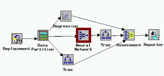
Classification Methods such as Decision Trees and Neural Networks are not effective to classify mortality status because of the disparate sample sizes.� The model shown in Figure One, constructed using SAS Enterprise Miner gives further information concerning the ability of patient laboratory values to predict length of hospital stay.� The model in the diagram (Figure 1) runs from left to right, with each icon representing a unique procedure in the analysis of the data.� Data are entered into the model.� Missing cells are replaced by the variable mean.� The data are then partitioned into training, testing, and validation stages.� A regression, decision tree, and neural network model are then run.�� The results for all procedures are given through the reporter icon.�

Figure 1. Model from SAS Enterprise Miner for length of stay

Pharmaceutical information was clustered using the SAS Text Miner tool.� These clusters were ranked by a pharmacist according to patient severity, by the complications of congestive heart failure (CHF) and chronic obstructive pulmonary disease (COPD), and finally by mortality rates.� This information was incorporated into a linear model to examine its effect on length of stay.�

Results

Patients undergoing open heart surgery have pre-admission blood testing, and a number of laboratory values are collected. Table 1 gives the relationship of patient laboratory values to length of stay.� It contains the coefficient estimates for a linear regression model. The patient laboratory values included in the model are hematocrit, white blood cell count, glucose, and creatinine. Two-way interactions were included in the model.� In particular, glucose appears to have a large effect (p=0.002).� However, the low R² value of .065 illustrates the need to include additional information in the model.� Adding pharmaceuticals does improve the model.� Pharmaceuticals the patient received while in the hospital were clustered using the Text Miner feature of SAS.�

Table 1.�

Linear Model for Length of Stay, Patient Laboratory Values

 

Variable	Estimate	St. Error	P-Value
Intercept	21.6	4.33	<.0001
Glucose	-.089	.03	.002
Hematocrit	-.24	.11	.03
Creatinine	-.51	.13	<.0001
White Blood Cell Count	-.33	.15	.03
Glucose*Hematocrit	.0014	.0007	.04
Glucose*Creatinine	.01	.002	<.0001
Glucose*White Blood Count	.003	.0009	.002
Hematocrit*Creatinine	.006	.003	.04
Hematocrit*White Blood	-.0002	.004	.94
Creatinine*White Blood	.029	.009	.002

 

Each cluster, shown in Table 2, contains pharmaceuticals commonly prescribed together.� These prescription combinations were then taken to pharmacist J. D. Cerrito who created a listing of possible health conditions for which the drugs in each cluster are commonly prescribed (personal communication, August 2003).� This pharmacist then ranked the clusters in order of probable severity.� Using information also contained in the dataset, the clusters were arranged in order of severity for the complications of CHF and COPD.� Severity was determined through an ordinal ranking of the percentage of patients in each category who suffered from the given condition.� Finally, the clusters were ranked according to frequency of mortality.� Again, the clusters were ordered, with the cluster having the greatest frequency of mortality having the greatest severity ranking.� The results, shown in Table 3, illustrate the importance of this pharmaceutical information on predicting a patient�s length of stay.� The R² value for this model is 0.12.� Because of its influence on pharmaceutical prescriptions, diabetes is added as a control.� The R² value was greatly improved from the 0.065 in the original model.�

Table 2.�

Description of Pharmaceutical clusters

Cluster ID	Frequency	Rank COPD	Rank CHF	Rank Mortality	Rank Pharmacist	Associated Diagnoses
1	88	2	2	9	8	IDDM (insulin-dependent diabetes) CHF COPD
2	306	7	5	3	10	ASC (Vascular disease) ASCUD (Athrosclorotic cardiovascular disease)
3	42	3	1	7	7	CHF NDDM (non-insulin dependent diabetes)
4	8	1	9	1	2	Allergy Vertigo COPD HTN (Hypertension)
5	8	10	10	10	1	Depression HTN Pain
6	23	9	8	6	6	Angina GERD (gastro-esophagial reflux disease) Vertigo
7	34	8	7	8	4	Hyperlipidemia Blood clot Depression Smoking cessation Infection IDDM
8	158	6	4	5	3	HTN Angina Blood Clot
9	225	5	3	2	9	Angina Pain Infection
10	348	4	6	4	5	HTN Pain GERD

Table 3.�

Linear Model of Length of Stay, Including Diabetes and Pharmaceutical Information

Variable	Estimate	T-Value	P-Value
Intercept	88.2	2.38	.02
Diabetes	5.1	.93	.35
Glucose	-.06	-1.10	.27
Hematocrit	-.54	-1.68	.09
Creatinine	1.95	1.33	.18
White Blood Cell Count	-.2	-.31	.76
Cluster by CHF	-7.5	-2.24	.03
Cluster by COPD	-7.54	-1.69	.09
Cluster by Mortality	-1.57	-1.21	.23
Cluster by Pharmacist	-6.68	-1.67	.09
Diabetes*Glucose	-.007	-.55	.58
Diabetes*Hematocrit	-.035	-.46	.65
Diabetes*Creatinine	-.0002	0	.99
Diabetes*White Blood Cell Count	.133	.86	.39
Diabetes*Cluster by CHF	-.45	-.95	.34
Diabetes*Cluster by COPD	.11	.28	.78
Diabetes*Cluster by Mortality	-.56	-1.59	.11
Diabetes*Cluster by Pharmacist	-.03	-.12	.91
Glucose*Hematocrit	.001	1.61	.11
Glucose*Creatinine	.013	5.17	<.0001
Glucose*White Blood Cell Count	.003	2.63	.009
Glucose*Cluster by CHF	.004	.95	.34
Glucose*Cluster by COPD	-.004	-1.1	.27
Glucose*Cluster by Mortality	-.002	-.72	.47
Glucose*Cluster by Pharmacist	-.002	-.66	.51
Hematocrit*Creatinine	-.0006	-.07	.95
Hematocrit*White Blood Cell Count	.0007	.11	.92
Hematocrit*Cluster by CHF	.036	1.3	.19
Hematocrit*Cluster by COPD	-.01	-.40	.69
Hematocrit*Cluster by Mortality	.024	1.22	.22
Hematocrit*Cluster by Pharmacist	.012	.68	.50
Creatinine*White Blood Cell Count	.0003	.01	.99
Creatinine*Cluster by CHF	-.08	-1.32	.19
Creatinine*Cluster by COPD	-.14	-1.41	.16
Creatinine*Cluster by Mortality	-.11	-1.35	.18
Creatinine*Cluster by Pharmacist	-.09	-2.00	.05
White Blood Cell Count*Cluster by CHF	-.02	-.36	.72
White Blood Cell Count*Cluster by COPD	.001	.03	.98
White Blood Cell Count*Cluster by Mortality	-.03	-.69	.49
White Blood Cell Count*Cluster by Pharmacist	-.0006	-.02	.99
Cluster by CHF*Cluster by COPD	.105	.41	.68
Cluster by CHF*Cluster by Mortality	.75	1.12	.26
Cluster by CHF*Cluster by Pharmacist	.025	.06	.95
Cluster by COPD*Cluster by Mortality	.029	.05	.95
Cluster by COPD*Cluster by Pharmacist	1.13	1.35	.18
Cluster by Mortality*Cluster by Pharmacist	0	.	.

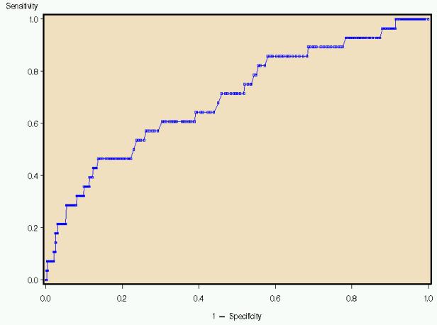
Figure 2 illustrates the Receiver Operating Characteristic (ROC) curve generated by a logistic model using the same terms listed for the linear model.� An ROC Curve is a plot of the true positive rate (sensitivity) against the false positive rate (specificity).� The larger the area under the curve (AZ value), the better the predictor. This model indicates the every increase in specificity results in a corresponding decrease in sensitivity, making it a poor modeling choice.� Indeed, because of the disparate sample sizes, logistic regression is often a poor modeling choice for this type of data.� A model that identifies all patients as low risk for mortality will be 96% accurate because 96% of the patients survive.� None of the terms were significant at the 0.05 level.

Figure 2. ROC Curve, logistic estimate of mortality status

Kernel density estimates the shape of the distribution of a particular variable by taking the proportion of data points that occur within a given interval and dividing by the length of that interval.� If a laboratory value is a good predictor of mortality, there will be an observable difference in the peaks of the distributions.� Figure 3 illustrates that patients who have a creatinine level greater than two are at higher risk for death than those patients with lower creatinine levels. The number 2 was chosen because it defines renal failure prior to surgery. Glucose levels in Figure 4 do not appear to differ between patients who survived and did not survive surgery.� The hospital has initiated a protocol to monitor and adjust glucose levels for patients before, during, and after surgery. The kernel density estimators indicate the success of the protocol. For other measures, a slight shift can be observed.� Patients with a white blood cell count higher than 6 have a slightly greater mortality risk (Figure Five).� Patients with a hematocrit level lower than 30 also have a slightly greater risk of mortality (Figure Six).

��������

Figure 3. Kernel density estimation, creatinine�� ���������������������������������������������������

Figure 4. Kernel density estimation, glucose

�

Figure 5. Kernel density estimation, white blood cell count

�

Figure 6. Kernel density estimation, hematocrit

Conclusion

The decision tree and neural networks are used to classify groups. The classifications were approximately equally successful in determining the patient�s length of stay.� The average squared error of these methods in the training phase is 55.� Unfortunately, in the testing phase this error rose to 280 depending on the specific method used.� As with linear regression, these values could probably best be reduced by adding other measures influencing patient care and complications of open heart surgery.� Other models must be defined to determine hospital quality. The standard linear and logistic regression models fit too poorly.�